Strange Overtones

Thanks to a familiarity with several flavors of mechanics – Newtonian, Lagrangian, Hamiltonian – I thought I had a good understanding of the vibration of a string, and I wasn’t expecting any surprises when I wanted to test a new audio interface to record the output of my digital piano. After having refreshed my memory with Tsuji and Müller’s Physics and Music [1], I knew that when I pressed the middle C, I expected a signal with a fundamental frequency1 at 262 Hz and overtones at integer multiples of that. Using a script that fetched the data, I plotted a spectrogram as I played. (I thought this would be a useful way to look at chords to visualize how they generate a series of overlapping overtones.) I planned to use this to do some live signal processing, but I never made it beyond recording a spectrum of that middle C:

Each instrument has a ‘fingerprint’ set by the ratios of the strengths of its overtones, this is called its timbre, and it’s what makes tones at the same pitch sound differently on each instrument. The spectrum above shows the timbre of a piano, but what was disconcerting to me was that the higher overtones started to drift away from the place where I expected them ($n \times 262~\mathrm{Hz}$, the vertical lines in the plot).
First I thought the sampling frequency I recorded at must have been slightly different, compressing or stretching the frequency axis a little. I tried rescaling the axis, but this messed up the presumptive frequency of the fundamental, so I gave up, and hypothesized that the audio interface must have been broken in some weird nonlinear way. It was only later, while reading some papers on piano tuning, I found out that there’s some stuff they don’t teach you about string vibration in undergrad.
Good Vibrations
The typical derivation of the equation of motion for a vibrating string goes something like this: the string is fixed on both ends, and held under tension by some force $T$. Under the assumption of a vibration amplitude that’s small compared to the wavelength, the vertical restoring force on a string element $dx$ can be related to tangent through the vertical angles on either end, $\alpha$ and $\beta$ (see figure below).

To make a connection with what’s to come, we also allow for an external load or force acting on $dx$ in the vertical direction, $q$; then, the equation of motion for the deviation of the string, $w(x, t)$, is given by:
\[T\frac{\partial^2 w}{\partial x^2} + q = \mu \frac{\partial^2 w}{\partial t^2},\]where $\mu$ is the linear density, such that $\mu dx$ is the element’s mass. After setting $q = 0$ and through a separation of variables, this results in the wave vectors ($k_n = \pi n/L$) and frequencies ($f_n = n f_0$, $f_0 = \frac{1}{2L} \sqrt{\frac{T}{\mu}}$) of the eigenmodes. The strings for middle C would typically have a radius of 0.57 mm, length of 0.67 m and at a tension of about 1 kN [2], which would result2 in a fundamental frequency of approximately 261 Hz.
We cannot understand the deviations in the frequency spectrum from this, but we can make an unrelated, remarkable observation: since there are over 200 strings in a typical piano, the weight equivalent of the total tension is around $20\times 10^3~\mathrm{kg}$, or two large elephants!
The problem is that, at high frequencies, piano wire starts to behave more like a rod rather than an ideal string. It does so because it has a finite stiffness, which can easily be observed by holding one end of some length of piano wire in your hand and letting the other end dangle free. Bending costs work (here done by gravity), and instead of making a right angle like an ideal, infinitely flexible wire, it will follow some curve. How do we describe this?
$I$ Bend Like This
Interestingly enough, this is a common problem in mechanical engineering [3], as the physics is identical to that of beams and columns – vital elements in buildings and bridges. The bending of a loaded beam is typically studied through the so-called Euler–Bernoulli equation, which describes how a beam bends in the presence of external forces or torques. Since we are primarily interested in studying the dynamics of a stiff string after it’s been hit with a felt hammer, it’s not useful to derive the static Euler-Bernoulli equation here. Instead, we’ll figure out how much energy is required to bend a (piece of) wire, and then use the principle of least action to derive the wave equation (the details of which have been relegated to the Encore below).
What is the bending energy of a stiff piece of wire, then? If it’s a simple material, the relative deformation (‘strain’) $\varepsilon$ is related to the stress $\sigma$ through Young’s modulus $E \equiv \sigma/\varepsilon$, which we’ll assume is constant. We can understand the strain as the amount by which a material stretches in the presence of stress: if we pull at a rope of length $L$, cross section $A$, and Young’s modulus $E$, with some force $F$, it will stretch to $L’ = \varepsilon L = F L / A E$. This stretching requires work: the taut rope is under some stress $\sigma = F/A = \varepsilon E$. The stretching energy density (energy per unit length) of a surface element $dA$, then, is the work required to bring this about. Integrating out from the stressless case, we can calculate this energy density as:
\[u_A = \int_0^\varepsilon \varepsilon' E \, d\varepsilon' = \frac{1}{2} E \varepsilon^2,\]which we should integrate over the entire cross-section and length of the wire to get the total stretching energy. We can obtain the strain $\varepsilon$ from a geometrical argument (also see the figure below) by considering a wire element $dx$. When this is being bent, there’s no net force pushing this left or right, meaning the stresses on the cross-section cancel, and its integral is zero: $\int \sigma \, dA = 0$. Furthermore, if the direction of bending is along the vertical $y$ axis, $\sigma = \sigma(y)$. Finally, if all deformations are small the stress is linear, meaning there is some $y_0$ such that $\sigma \propto (y-y_0)$. This $y_0$ (together with the out-of-plane axis) defines the ‘plane of bending’ where the stress vanishes [3]. Without loss of generality, we translate the y axis such that $y_0 = 0$ without loss of generality.

The strain is given by the change in length of an element $dx$, and is a function of the vertical coordinate $y$. Using similar arguments as when deriving the wave equation for a flexible string, we can see
\[\\ \begin{align} dx' = \varepsilon dx &= y \left[ \tan(\beta) - \tan(\alpha) \right] \\ &= y \left[ \frac{dw}{dx}(x+dx) - \frac{dw}{dx}(x) \right]. \end{align} \\\]The presence of $dx$ suggests we can connive with some calculus to obtain (after dividing it on both sides):
\[\varepsilon = y \frac{d^2 w}{dx^2}.\]The bending energy of this wire element, then is:
\[\\ \begin{align} u_b &= \int u_A \,dA \\ &= \frac{1}{2} E \int \varepsilon^2 \,dA \\ &= \frac{1}{2} E \int y^2 \left( \frac{d^2w}{dx^2}\right)^2 \, dA \\ &= \frac{1}{2} E I \left( \frac{d^2w}{dx^2}\right)^2. \end{align} \\\]In the last step we’ve used the fact that $w(x)$ doesn’t depend on $y$, and we’ve defined $I = \int y^2 \, dA$; this is also called the bending moment or the second moment of the area. A standard string has a circular cross-section with radius $r$, in which case $I = \pi r^4/4$.
We can use this energy density to calculate the action, which we use in the Encore below to derive the equation of motion for the string. The general result is given there, but if there is no external force acting on the string, we find the wave equation for stiff wires (or the dynamic Euler-Bernoulli equation for a taut string, if you wish):
\[\boxed{ EI \frac{\partial^4 w}{\partial x^4} - T \frac{\partial^2 w}{\partial x^2} = -\mu \frac{\partial^2 w}{\partial t^2}.}\]This is relatively easy to solve through a separation of variables; if we do so we find the new, anharmonic eigenfrequencies:
\[f_n = nf_0 \sqrt{1 + \frac{EI}{T}\left( \frac{n\pi}{L} \right)^2}.\]Of cords and chords
Since the spatial part of the solutions of ideal string [$\sim\!\sin(k_n x)$] is an eigenfunction of the $\partial^4/\partial x^4$ operator, its functional shape is maintained by the differential equation given above (although its eigenvalues change, resulting in frequency shifts). This means that, if we know the initial condition $w(x, t = 0)$, we can calculate its overlap with a basis of sinusoids, which will give us the time-dependent oscillation, which we can use to synthesize a tone (although this won’t sound like a piano, since we do not account for its frame and soundboard, which are also important for its acoustic properties).
We can use this to generate a chord; setting the parameters3 of three strings such that they produce the C major chord (C-E-G), we get the following signal (click the spectrogram to play the sound):
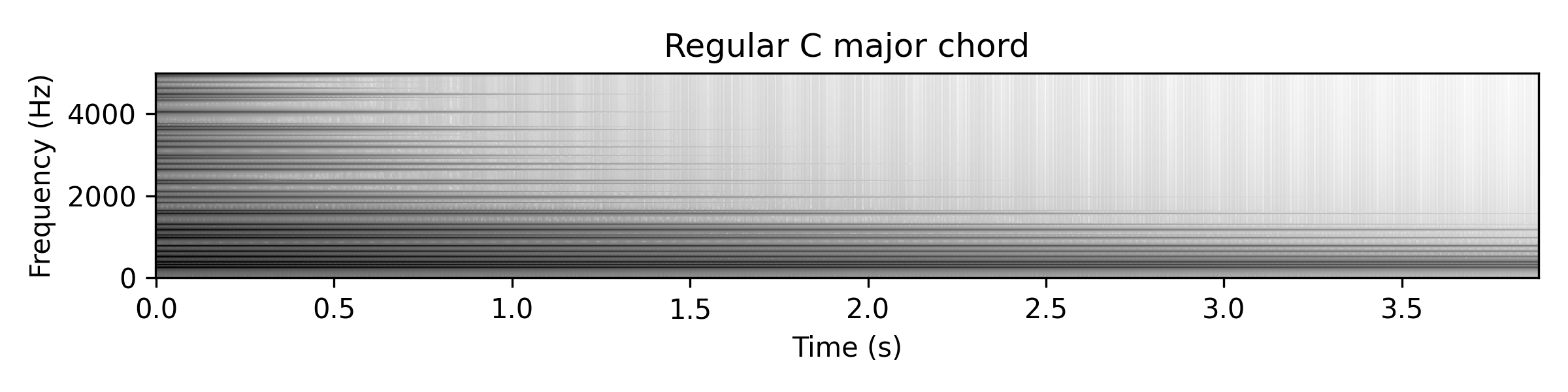
It sounds a bit like a Rhodes piano! Since this is all synthesized, we can also create a set of artificial strings which are very flexible and for which bending costs no energy ($E = 0$). Visually it’s very difficult to see the difference (there are some harmonics above $4~\mathrm{kHz}$ which are different in the first $0.5~\mathrm{s}$ before damping out – click the spectrogram to play the sound):
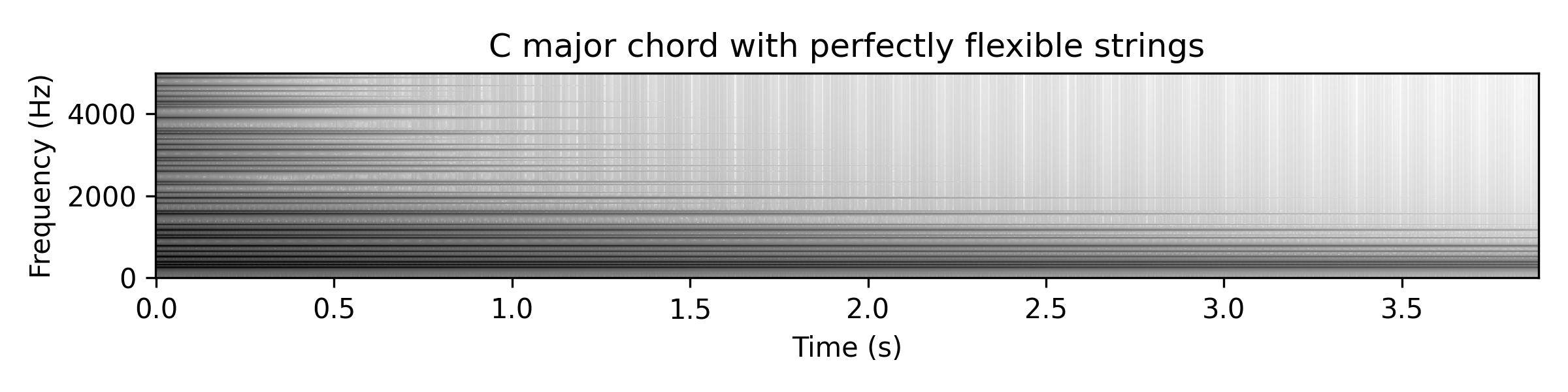
It can also be quite hard to hear the difference. I have to play both chords a few times in a row to tell that the second one is slightly (slightly!) flat compared to the first one, which is to be expected since the anharmonicity pushes frequency components up.
“It sounded great, but it could’ve used a little more 🔔”
The difference between the two chords generated above may be subtle, but if we artificially increase the elastic modulus we can learn something interesting. In the following spectrogram $E$ has been increased by a factor 500; the plot looks significantly different because the anharmonicity is so much larger (click it to play the sound):
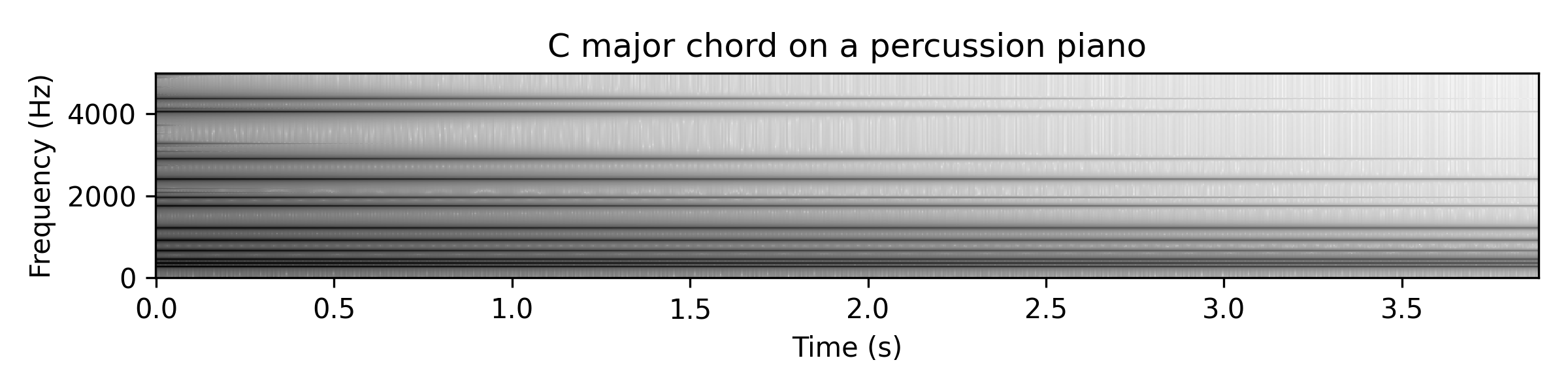
It sounds much more like a bell or a gong than like a string instrument. This isn’t strange – all string and wind instruments can (to some approximation) be described by a one-dimensional wave equation (be it describing a string or a column of air), resulting in an even series of overtones. Most percussion instruments, meanwhile, have much more complicated geometries, meaning the frequencies of their eigenmodes don’t stack up in a neat harmonic series [1]. By increasing the material stiffness, we are turning a string into a rod, and a piano into a percussion instrument!
String anharmonicity is only a part of piano acoustics, and there are many more interesting considerations that go into piano design. A standard 88-key instrument spans about 7 octaves, which is a factor $2^7 = 128$ in frequency. To avoid having to deal with strings that differ by more than two orders of magnitude in length, bass strings are typically thicker. This also increases their anharmonicity, though, so to keep this in check they are wound with copper wire to increase their weight density $\mu$ without increasing the anharmonicity through $I$.
What’s charming about string anharmonicity is that it connects material typically reserved for engineering courses (the physics of beams and columns) to something as elementary as string vibration, introducing some non-idealities along the way to understand the behavior of this real-world system. I have a feeling that undergraduate-me would have considered this an interesting special topic in my undergraduate dynamics course.
Encore: Equations for Strings
Before going through Feynman’s lecture on the principle of least action [5], I was always a bit intimidated by the Lagrangian approach to mechanics. I hope this problem can serve as evidence that this apprehension is unjustified, and that, in fact, it can be an elegant approach to dynamics.
The goal is to obtain the equation of motion for a string described by $w(x, t)$; to do so we need to minimize the action, so we need both the kinetic end potential energy. The kinetic energy density of a string element with weight density $\mu$ is given by:
\[t = \frac{1}{2}\mu \left(\frac{\partial w}{\partial t}\right)^2.\]As for the potential energy density, we like to keep things general, and so we assume the string is subjected to an external force with density $q$, which performs work ($qw$) that causes the string to bend.4 If the string has nonzero stiffness, bending it will cost energy, the energy of which we’ve derived above. The string, finally, is held under some tension $T$. What is the potential energy associated with this? At rest, there is none, but if the string deviates from its rest position by $w(x)$ work must be done to overcome the tension.
Derivations of the wave equation in a string, typically contain an intermediate result that states that the vertical restoring force density is given by:
\[f_y = T \frac{\partial^2 w}{\partial x^2}.\]The work, then, performed to pull the string to this position, is:
\[\\ \begin{aligned} u_T &= T \int_0^w \frac{\partial^2 w'}{\partial x^2} \, dw' \\ &= T \frac{\partial^2}{\partial x^2} \int_0^w w' \, dw' \\ &= \frac{T}{2} \frac{\partial^2 w^2}{\partial x^2} \\ &= T\left[ \left(\frac{\partial w}{\partial x}\right)^2 + w \frac{\partial^2 w}{\partial x^2} \right]. \end{aligned} \\\]Combining all the contributions to the potential energy density, we find:
\[u = \frac{1}{2} E I \left( \frac{\partial^2 w}{\partial x^2} \right)^2 + T\left[ \left(\frac{\partial w}{\partial x}\right)^2 + w \frac{\partial^2 w}{\partial x^2} \right] + q w.\]We now turn to the action integral that we should minimize, which becomes:
\[\\ \begin{aligned} S &= \int_{t_1}^{t_2} \int_0^L (t - u) \, dx \,dt \, \\ &= \int_{t_1}^{t_2} \int_0^L \mathcal{L}\left[ x, t, w, \partial w/\partial t, \partial w/\partial x, \partial^2 w/\partial x^2 \right] \, dx \,dt, \end{aligned} \\\]where it’s implied that $w = w(x, t)$. The system has one degree of freedom – $w(x,t)$ – which depends on two variables; the Lagrangian $\mathcal{L}$, in turn, contains higher derivatives of $w$ which means we need to use the Euler–Lagrange equation that takes accounts for these. Only keeping the nonzero terms, and using $\dot{w}$ and $w’$ to denote differentiation with respect to $t$ and $x$, respectively, this is:
\[\frac{\partial \mathcal{L}}{\partial w} - \frac{\partial}{\partial t} \frac{\partial \mathcal{L}}{\partial \dot{w}} - \frac{\partial}{\partial x} \frac{\partial \mathcal{L}}{\partial w'} + \frac{\partial^2}{\partial x^2} \frac{\partial \mathcal{L}}{\partial w''} = 0.\]If we evaluate this, we find the Euler-Bernoulli beam equation for a string under tension:
\[EI \frac{\partial^4 w}{\partial x^4} - T \frac{\partial^2 w}{\partial x^2} = -\mu \frac{\partial^2 w}{\partial t^2} - q.\]Setting $EI = 0$ reduces this to the familiar wave equation for strings, while setting $T = 0$ results in the dynamic Euler-Bernoulli beam equation which is common in mechanical engineering. (The form given here is restricted to so called ‘prismatic beams’ for which $E$ and $I$ are constants. Other cases can easily be accommodated by keeping them inside of the derivatives of the Euler-Lagrange equation.)
References
[1] K. Tsuji and S.C. Müller, Physics and Music, Springer Nature (2021)
[2] H. Fletcher, Normal Vibration Frequencies of a Stiff Piano String, The Journal of the Acoustical Society of America 36 (1964), 203–209
[3] J.M. Gere and B.J. Goodno, Mechanics of Materials, Seventh Edition, Cengage Learning (2009)
[4] N. Giordano, Explaining the Railsback stretch in terms of the inharmonicity of piano tones and sensory dissonance, The Journal of the Acoustical Society of America 138 (2015), 2359–2366
[5] R.P. Feynman et al., The Feynman Lectures on Physics, Chapter 19: The Principle of Least Action (2013)
Notes
-
The piano in this experiment is tuned so that the A above middle C is at 440 Hz. Since going down an octave halves the frequency, this means that the A below middle C is at 220 Hz. Going up by three steps in equal temperament, middle C is at $220 \cdot 2^{3/12}~\mathrm{Hz} \approx 262~\mathrm{Hz}$. ↩
-
Assuming that the string is made out of steel wire with a density of 8000 kg/m$^3$. ↩
-
For the C string, by visual fitting to the recorded spectrum included above: $L = 0.675~\mathrm{m}$, $T = 1015~\mathrm{N}$, $E = 180~\mathrm{GPa}$, and assuming a circular cross-section (for which $I = \pi r^4/4$) with $r = 0.57~\mathrm{mm}$. The E and G strings are obtained by decreasing $L$ by a factor of $5/4$ and $3/2$, respectively. ↩
-
Note that, especially in mechanical engineering literature on beams, $q$ is often referred to as a load, and the convention is that $q > 0$ if the load exerts a downward force. Here we take the opposite convention, meaning that $q > 0$ implies a force pointing in the positive vertical direction (upwards), more in line with its vectorial nature. ↩