Much has been made of people coughing during classical concerts. An economist has observed that the rate at which people cough during a concert is roughly twice that of the baseline, and has hypothesized that, among other reasons, they do so in order to express their disapproval with the performance while barely staying within the confines of the etiquette in Concert Hall [1]. Coughing avalanches (the phenomenon where one cough leads to two leads to more), are explained as fellow concertgoers reaching mutual agreement that the performance isn’t what they expected.

While these explanations are quite original, I think they take a needlessly negative view of an audience that ultimately attends a performance of its own volition. I have no evidence either way, but I would argue it is more likely the strict concert etiquette that’s to blame. The ‘rule’ that there’s applause at the end of a piece but not between movements is sufficient to keep the uninitiated on their toes, for instance. ‘Was this merely a few rests, or the end of a movement? Which movement are they playing now? Is it the last one? Why is the conductor still holding their baton aloft? Surely there’s applause now, right? Right?’

It doesn’t take much to imagine audiences getting pretty neurotic about the ‘no cough rule,’ not unlike a child that has to go to the bathroom but gets told to hold it in a little while longer. Everyone settles down in their seats, the woodwinds blow something close enough to 440 Hz to start tuning, then the strings join, and, as if it were none other than Pavlov himself conducting, some throats start to itch. There’s a cough, maybe two. ‘Perhaps I should cough preemptively, while it’s still allowed,’ a few think, and proceed to clear their throat. Then, later – the performance is well underway – a quiet passage arrives. ‘How embarrassing would it be if someone coughed now?’ crosses a few minds, and then: ‘Hold on, there’s that bedeviled itch again!’

This also happens between movements. While clapping is verboten, coughing is certainly preferred between rather than during movements, and so there are plenty of recordings where the hive decides to let it rip. Listen, for instance, to the tussis collectivus at the end of the first movement in this recording of Mozart’s Haffner Symphony in Amsterdam. And look at that disappointment:

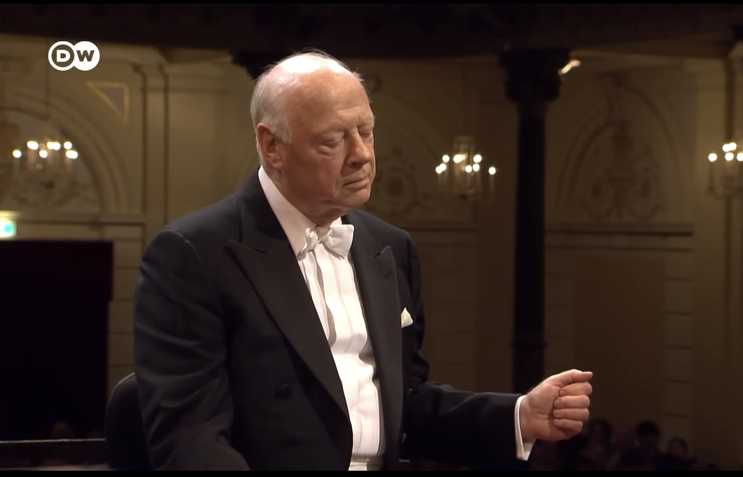
A disappointed Bernie, courtesy of DW.

As someone who has been studying stochastic processes in quantum mechanical systems for the past couple of years I find this very interesting. While an orchestra is, in essence, a phase locked loop with the conductor serving as its master oscillator, the audience has an enormous potential to generate noise and disruption (see Figure above). What is the $g_2(t)$ of these coughs? Are they bunched or antibunched? Should we think of it as superradiance?

While I have no definitive answer to these questions, I can formulate the simplest description that others will have to improve upon – call it the null hypothesis of tussis collectivus.

$H_0$: Coughing heard before a concert and in between movements is a Poisson process.

What this means is that the probability of hearing a cough at some time $t$ is constant, and that it does not depend on whether a cough has been heard at some time $t’ < t$. This is one of the simplest stochastic processes that involve discrete arrival times. A consequence is that the time between coughs is given by an exponential distribution¹, which has a probability density function

\[f(\tau; \lambda) = \lambda e^{-\lambda \tau},\]

where $\lambda$ is the rate, and which is defined for $\tau \geq 0$ [2]. The reason this is called a Poisson process is that the number of clicks observed during a particular interval $T$ are described by a Poisson distribution with mean $\lambda T$.

We can apply this to the coughs heard between movements of the Haffner Symphony linked above, and ask: what is the most likely value of $\lambda$ underlying this process, and how probable is it in general that the coughs we hear are produced by a Poisson process? Here’s the clip:

In order to do this, I’ve tried to time the moments where people cough (at some point there’s significant overlap and it’s difficult to be accurate). There’s about thirteen of them in a twelve-second window – when plotted on a line it looks like this:

If we let $\tau_i = t_{i+1} - t_i$ be the time between the $i$ and $(i+1)^\mathrm{th}$ cough, the probability that a sequence of $N + 1$ coughs was generated by a Poisson process with rate $\lambda$ equals:

\[P\left(\vec{\tau}|\lambda\right) = \prod_{i=1}^{N} \lambda e^{-\lambda \tau_i}.\]

What is the most likely value of $\lambda$, though? In a Bayesian turn, we can flip this probability around [3], and ask: how likely is it that we are dealing with a Poisson process with rate $\lambda$ here? Since we don’t have any useful prior knowledge on $\lambda$ this results in the likelihood $f_\lambda(\vec{\tau}) \propto P\left(\vec{\tau}|\lambda\right)$.

To avoid having to deal with the very small numbers that we get when multiplying a series of small-ish numbers, it’s convenient to take the logartihm of this expression and work with the log-likelihood. As an added bonus it turns the product in a sum and we get rid of the exponential:

\[\mathcal{L}_\lambda \equiv \ln\left[ f_\lambda(\vec{\tau}) \right] \propto N \ln(\lambda) - \lambda \sum_{i=1}^{N} \tau_i.\]

Maximizing this, we find the most probable value of $\lambda$ (aka the maximum likelihood estimate). Solving $d\mathcal{L}_\lambda/d\lambda = 0$ we obtain (perhaps unsurprisingly):

\[\lambda_\mathrm{MLE} = \frac{N}{\sum_{i = 1}^{N} \tau_i} \approx 1.05~\mathrm{s^{-1}},\]

which we can recognize as the inverse of the mean time between coughs (which explains why $\lambda$ is called the rate). Finally it would be useful to get an idea of how confident we should be in this estimate (to put an error bar on it, as it were). It helps to plot $\mathcal{L}_\lambda$, the dot here represents $\lambda_\mathrm{MLE}$:

Qualitatively, we should be confident in our estimate of $\lambda_\mathrm{MLE}$ if $\mathcal{L}_\lambda$ changes strongly if we take a step left or right. This is the case if the curve is very sharp. One way of expressing this is through the second derivative of the curve, also known as the Fisher information. It gives us an estimate of the average error:

\[\sigma^2 = \left[ -\frac{d^2\mathcal{L}_\lambda}{d\lambda^2} \right]^{-1}.\]

For this problem, it turns out that², $\sigma = \lambda/\sqrt{N}$, meaning we have a relative error of $\sigma/\lambda \approx 0.3$ for $N = 12$ time intervals.

So far we have been working under the assumption that the time intervals are exponentially distributed, and this comes with some limitations. Since it implies that the probability of registering a cough at any time is independent of what came before, it would never allow us to explain correlations, so no true tussis collectivus. It does, however, give us a baseline to compare more complicated models to, but doing this, as we say, is an interesting direction for future research.

References

[1] A. Wagener, Why Do People (Not) Cough in Concerts? The Economics of Concert Etiquette, ACEI working paper series, AWP-05-2012 (2012). (link)

[2] A. Kiely, Exact classical noise master equations: Applications and connections, Europhysics Letters 134 (2021), 10001. (link)

[3] H. Liu and L. Wasserman, Statistical Machine Learning, Chapter 12: Bayesian Inference (2014). (link)

Notes

This may seem at odds with the claim that the coughs are uncorrelated: it would suggest that having heard a cough at time $t_1$ it would allow you to predict the arrival time of the next one, $t_2$. While $t_2 - t_1$ is exponentially distributed, an analysis would show that this prediction doesn’t in fact rely on having the knowledge of there having been a cough at $t_1$ – this is for another time, though. ↩
Fortunately not contradicting the central limit theorem and so on. ↩